A Graph Convolution Network in SageMaker
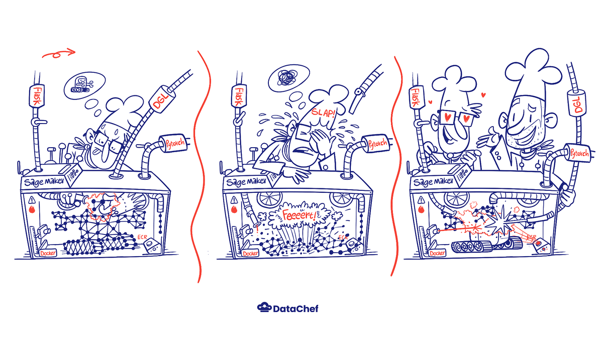
Introduction Graph neural networks provide a more flexible paradigm for machine learning models by explicitly accounting for entities and their relationships through neural networks. For example, It is easier to model a real problem with graphs in so...
Introduction
Graph neural networks provide a more flexible paradigm for machine learning models by explicitly accounting for entities and their relationships through neural networks. For example, It is easier to model a real problem with graphs in social sciences or networks. As a matter of fact, graphs are ubiquitous in machine learning and computer science. For instance, an image can take the form of a graph where each pixel is a node connected to each one of its neighbors by an edge. Despite the fact that these grid shapes enjoy regular structures, most structures in real life are considerably more complex. In this sense, GNNs generalize classic models such as convolutional neural networks, LSTMs, etc., to tackle a larger class of problems.
This post will walk you through a classification problem defined over a graph which is modeled by a graph neural network step-by-step. It will make use of Amazon SageMaker, Deep Graph Library, and PyTorch.
The source of this project is available in our GitHub repository.
Graph Convolution Networks
If you know about convolution layers in convolutional neural networks (CNNs), the function of convolution in a graph convolution network (for short: GCN) is similar. It refers to convolving the input signal by a set of neurons (which consists of weights that are shared across the input domain) that are commonly known as filters or kernels. Filters allow CNNs to gather features from nearby cells as they slide across the image.
These models use a similar approach in that they learn the features by looking at the neighboring nodes. One of the main differences between CNNs and GCNs is that in a CNN, the underlying image also has an ordered grid structure, while in GCNs, nodes normally aren’t ordered.
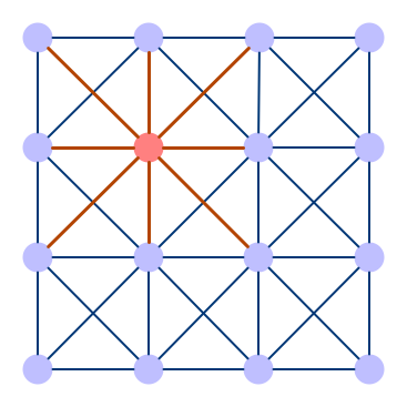
Convolutional Neural Network
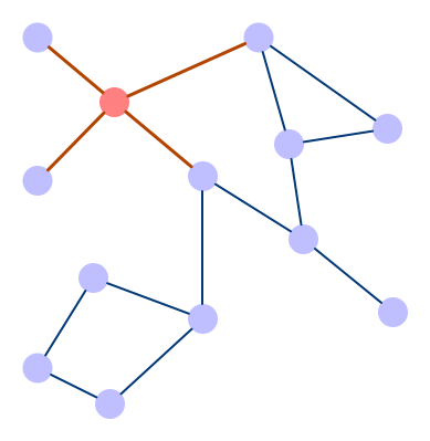
Graph Convolutional Network
Dataset
The purpose of this post is to illustrate how GCNs can be implemented in SageMaker using DGL. We skip the preprocessing phase and use one of DGL’s preprocessed datasets.
A collection of benchmark datasets is included in the DGL package, which is divided into three main categories (see documentation for details):
Node Prediction (node classification)
Edge Prediction
Graph Prediction (graph classification)
For this project, the CoraFull dataset was chosen as an example of how the architecture of a neural network for classification is built on top of Amazon SageMaker using PyTorch and DGL.
SageMaker Setup
Git Repository
Developing in both SageMaker notebook and your IDE (local machine) have their privileges. Besides that, it is always necessary to keep track of your code. To do so, before creating the notebook, we need to add a repository under the SageMaker → Notebook → Git repositories.
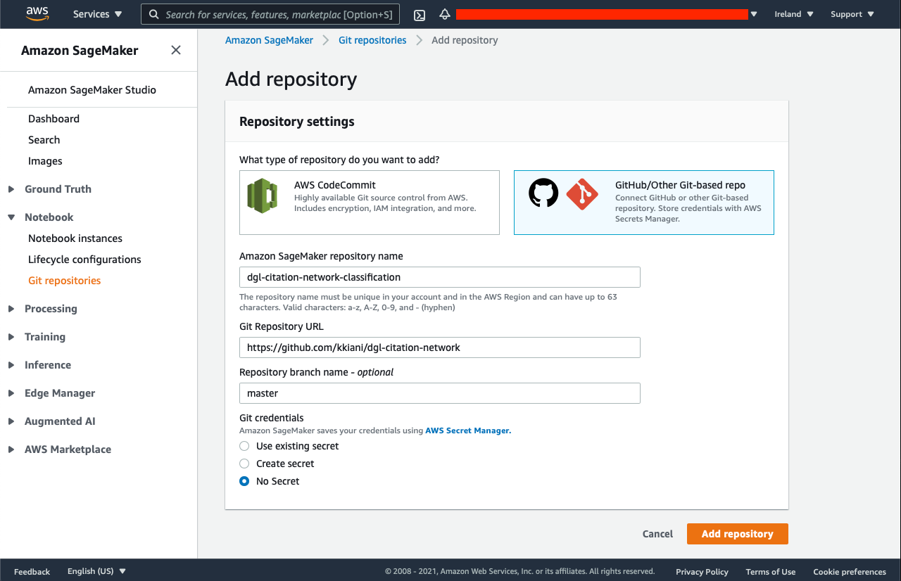
To prevent any risk, you can select “No Secret” under Git credentials to not to save your GitHub’s username and passwords. You can create a specific access token only for this repository from your GitHub profile → Settings → Personal access tokens → Generate new token, and use it later in SageMaker JupyterLab to push to your repository.
Deep Graph Library
Deep Graph Library (DGL) is an open-source python framework that has been developed to deliver high-performance graph computations on top of the top-three most popular Deep Learning frameworks, including PyTorch, MXNet, and TensorFlow. DGL is still under development, and its current version is 0.6.
Overview of DGL - DGL 0.4.3post2 documentation
Dataset loader
Every dataset in the DGL package inherits from dgl.data.DGLDataset. This base class formulates utilities for downloading, processing, saving, and loading data from external resources. Every dataset may contain one or more graphs.
The CoraFull dataset is one of the built-in DGL datasets, which is a graph representation of scientific papers under 70 categories. Each node represents a paper, and the edges between nodes are the citation network. The following are statistics of this dataset:
Nodes: 19,793
Edges: 126,842
Number of Classes: 70
Node feature size: 8,710
The class labels in this dataset are stored in “ndata_scheme” properties with the key of “label”. They are in tensor format in which their index corresponds to the node’s ID.
>>> from dgl.data import CoraFullDataset
>>> dataset = CoraFullDataset()
>>> graph = dataset[0]
>>> graph
Graph(num_nodes=19793, num_edges=126842,
      ndata_schemes={'label': Scheme(shape=(), dtype=torch.int64), 'feat': Scheme(shape=(8710,), dtype=torch.float32)}
      edata_schemes={})
>>> dataset.num_classes  # number of classes for each node.
70
>>> graph.ndata['feat']  # get node feature
tensor([[0., 0., 0.,  ..., 0., 0., 0.],
        [0., 0., 0.,  ..., 0., 0., 0.],
        [0., 0., 0.,  ..., 0., 0., 0.],
        ...,
        [0., 0., 0.,  ..., 0., 0., 0.],
        [0., 0., 0.,  ..., 0., 0., 0.],
        [0., 0., 0.,  ..., 0., 0., 0.]])
>>> graph.ndata['label']  # get node labels
tensor([ 0,  0,  0,  ..., 52, 59, 55])
Graphs
Graphs in DGL inherit from dgl.DGLGraph. All graphs in DGL are directed by defaults, and to make indirect graphs, you need to create edges both from $u$ to $v$ and $v$ to $u$. It is also possible to use dgl.to_bidirected() function to turn directed one to undirected one more efficiently.
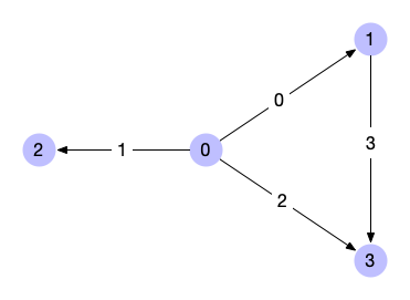
Example of a directed graph
The code snippet below represents the graph in the above picture:
>>> import dgl
>>> import torch as th

>>> # edges 0->1, 0->2, 0->3, 1->3
>>> u, v = th.tensor([0, 0, 0, 1]), th.tensor([1, 2, 3, 3])
>>> g = dgl.graph((u, v))
>>> print(g) # number of nodes are inferred from the max node IDs in the given edges
Graph(num_nodes=4, num_edges=4,
      ndata_schemes={}
      edata_schemes={})

>>> # Node IDs
>>> print(g.nodes())
tensor([0, 1, 2, 3])
>>> # Edges from nodes u to nodes v
>>> # edges 0->1, 0->2, 0->3, 1->3
>>> print(g.edges())
(tensor([0, 0, 0, 1]), tensor([1, 2, 3, 3]))
>>> # Edge end nodes and edge IDs
>>> print(g.edges(form='all'))
(tensor([0, 0, 0, 1]), tensor([1, 2, 3, 3]), tensor([0, 1, 2, 3]))

>>> # If the node with the largest ID is isolated (meaning no edges),
>>> # then one needs to explicitly set the number of nodes
>>> g = dgl.graph((u, v), num_nodes=8)
Node features, labels and edge features can be set or accessed through the ndata and edata properties respectively.
>>> import dgl
>>> import torch as th
>>> g = dgl.graph(([0, 0, 1, 5], [1, 2, 2, 0])) # 6 nodes, 4 edges
>>> g
Graph(num_nodes=6, num_edges=4,
      ndata_schemes={}
      edata_schemes={})
>>> g.ndata['x'] = th.ones(g.num_nodes(), 3)               # node feature of length 3
>>> g.edata['x'] = th.ones(g.num_edges(), dtype=th.float32
)  # scalar float feature
>>> g
Graph(num_nodes=6, num_edges=4,
      ndata_schemes={'x' : Scheme(shape=(3,), dtype=torch.float32)}
      edata_schemes={'x' : Scheme(shape=(,), dtype=torch.int32)})
>>> # different names can have different shapes
>>> g.ndata['y'] = th.randn(g.num_nodes(), 5)
>>> g.ndata['x'][1]                  # get node 1's feature
tensor([1., 1., 1.])
>>> g.edata['x'][th.tensor([0, 3])]  # get features of edge 0 and 3
    tensor([1, 1], dtype=torch.int32)
Splitting Dataset
Because our dataset in GNNs now takes the form of a graph and not a tabular structure, we need a different function of splitting the dataset from typically used scikit-learn train-test split.
Masking is commonly applied to edge features, node features, and labels on split nodes during model training, testing, and validation. The split_dataset function returns masked indices related to what is passed as an argument.
from dgl.data.utils import split_dataset

# Getting dataset
dataset = CoraFullDataset()
graph = dataset[0]
# ... some other codes

# Splitting dataset
train_mask, val_mask = split_dataset(graph, [0.8, 0.2])

# Training
for epoch in range(epochs):
    # ... some other codes

    train_acc = (labels[train_mask.indices] == pred[train_mask.indices].argmax(1)).float().mean()
    val_acc = (labels[val_mask.indices] == pred[val_mask.indices].argmax(1)).float().mean()
PyTorch Integration
Many of the state-of-the-art graph convolutional layers are now natively implemented in DGL’s latest version.
dgl.nn - DGL 0.4.3post2 documentation
GraphConv implements the mechanism of graph convolution in PyTorch, MXNet, and Tensorflow. Also, DGL’s GraphConv layer object simplifies constructing convolutional models through the stack of GraphConv layers.
import torch as th
import torch.nn as nn
import torch.nn.functional as F
from dgl.nn import GraphConv

class GraphConvolutionalNetwork(nn.Module):
    def __init__(self, in_feat, h_feat, out_feat):
        super().__init__()

        self.gcl1 = GraphConv(in_feat, h_feat)
        self.relu = nn.ReLU()
        self.gcl2 = GraphConv(h_feat, out_feat)

    def forward(self, graph, feat_data):
        x = self.gcl1(graph, feat_data)
        x = self.relu(x)
        x = self.gcl2(graph, x)

        return x
Saving and Loading Graphs
Since we train our model on a specific graph, we need to also save that graph for later use.
import os
from dgl.data.utils import save_graphs,

# The SageMaker default system path for saving and loading model artifacts.
model_dir = '/opt/ml/model'

save_graphs(os.path.join(model_dir, 'dgl-citation-network-graph.bin'), graph)
import os
from dgl.data.utils import load_graphs
import torch as th

model_dir = '/opt/ml/model'

glist, label_dict = load_graphs(os.path.join(model_dir, 'dgl-citation-network-graph.bin'))
graph = glist[0]
Training
It is the train file’s responsibility to create a model from what we’ve defined in model.py. We begin the training loop in the training file like every other PyTorch script, but with three important differences:
The graph should also be passed through our model along with the inputs.
For loss function, which computes the difference between predicted labels and actual labels, the masked training indices are considered only.
Also, the validation and train accuracies are computed using only the corresponding indices.
#!/usr/bin/env python

import os, json

import torch as th
import torch.nn.functional as F

from dgl.data import CoraFullDataset
from dgl.data.utils import split_dataset, save_graphs, load_graphs

from model import GraphConvolutionalNetwork

def main():
    # Setup Variables
    config_dir = '/opt/ml/input/config'
    model_dir = '/opt/ml/model'

    with open(os.path.join(config_dir, 'hyperparameters.json'), 'r') as file:
        parameters_dict = json.load(file)

        learning_rate = float(parameters_dict['learning-rate'])
        epochs = int(parameters_dict['epochs'])

    # Getting dataset
    dataset = CoraFullDataset()
    graph = dataset[0]
    features = graph.ndata['feat']
    labels = graph.ndata['label']

    # Splitting dataset
    train_mask, val_mask = split_dataset(graph, [0.8, 0.2])

    # Creating Model
    model = GraphConvolutionalNetwork(features.shape[1], 16, dataset.num_classes)
    optimizer = th.optim.Adam(model.parameters(), lr=learning_rate)

    # Training
    for epoch in range(epochs):
        pred = model(graph, features)
        loss = F.cross_entropy(pred[train_mask.indices], labels[train_mask.indices].to(th.long))

        train_acc = (labels[train_mask.indices] == pred[train_mask.indices].argmax(1)).float().mean()
        val_acc = (labels[val_mask.indices] == pred[val_mask.indices].argmax(1)).float().mean()

        optimizer.zero_grad()
        loss.backward()
        optimizer.step()

        print(f'Epoch {epoch}/{epochs} | Loss: {loss.item()}, train_accuracy: {train_acc}, val_accuracy: {val_acc}')


    # Saving Graph
    save_graphs(os.path.join(model_dir, 'dgl-citation-network-graph.bin'), graph)

    # Saving Model
    th.save(model, os.path.join(model_dir, 'dgl-citation-network-model.pt'))

if __name__ == '__main__':
    main()
Serving
Once we have trained our model, it is time to provide an API so users and developers can make real-time inferences. SageMaker has an architecture for serving Machine Learning models. To make an inference in SageMaker you need to provide exactly two API with a web framework of your choice.
Ping (GET)–It is called by SageMaker to ensure the API is available and live. It takes no arguments and returns 200 if everything is OK. The message body must be an empty string and the request timeout is 2 seconds for this API.
Invocation (POST) - it is used by developers and users to make predictions. It must accept a text/csv file of request ids as an argument and return predictions for those ids. There is a timeout of 60 seconds for this API, which means we have 60 seconds to process all the data we receive and do all the computations before responding to this request.
Serving Prediction using Flask
Flask is a simple, easy-to-use mini framework for implementing APIs. It doesn’t take much boilerplate code to get a simple app running.
import os
from dgl.convert import graph
import pandas as pd
from io import StringIO

from dgl.data.utils import load_graphs
import torch as th

import flask
from flask import Flask, Response

model_dir = '/opt/ml/model'
graph_dir = '/opt/ml/input/data'

glist, label_dict = load_graphs(os.path.join(model_dir, 'dgl-citation-network-graph.bin'))
graph = glist[0]
model = th.load(os.path.join(model_dir, 'dgl-citation-network-model.pt'))
features = graph.ndata['feat']
pred = model(graph, features)

app = Flask(__name__)

@app.route("/ping", methods=["GET"])
def ping():
    return Response(response="\\n", status=200)

@app.route("/invocations", methods=["POST"])
def predict():
    if flask.request.content_type == 'text/csv':
        data = flask.request.data.decode('utf-8')
        s = StringIO(data)
        data = pd.read_csv(s, header=None)
        response = pred[data.values]
        response = str(response)
    else:
        return flask.Response(response='CSV data only', status=415, mimetype='text/plain')

    return Response(response=response, status=200)

if __name__ == '__main__':
    app.run(host='0.0.0.0', port=8080)
Batch Transform
Sometimes it is more convenient to make an inference on a large amount of data once in a while and save the output for future use instead of creating an endpoint and making the same computations every time.
Batch transform automatically manages the processing of large datasets within the limits of specified parameters.—AWS Documentations
The batch transform mode is not much different from deploying the API. In our Jupyter Notebook, we call transform(), and pass the S3 CSV file as its argument. SageMaker creates and runs the serve container and sends the CSV file to the /invocation API. Once SageMaker receives the response, it saves the output in another S3 bucket, deletes the endpoints, and stops serving to prevent charging.
import sagemaker
from sagemaker.estimator import Estimator

es = Estimator(
    role=sagemaker.get_execution_role(),
    image_uri='<PATH TO YOUR ECR REPO>',
    instance_type='ml.m5.large',
    instance_count=1,
    hyperparameters={
        'epochs': 100,
        'learning-rate': 0.01
    }
)

sess = sagemaker.Session()
prefix = 'kiarash/dgl-citation-network'

batch_input = sess.upload_data(path='../data.csv', key_prefix=prefix + '/batch')

es_transformer = es.transformer(
    instance_count=1,
    instance_type='ml.m5.large'
)

es_transformer.transform(
    batch_input,
    content_type='text/csv',
    wait=True,
    logs=True
)
Containarization
Docker empowers SageMaker to isolate every project’s configurations and its dependencies. Docker is available through the JupyterLab Terminal and Jupyter Notebook.
You can pull, commit or create a whole new image inside the docker. However, the docker image repositories and it’s all configurations will be reset by shutting down the Notebook to save space.
Making Dockerfile
It is easy to end up with big containers in docker, and it is always cost-efficient to keep our docker containers as small as possible. To do so, we keep in mind these points:
We start with Docker image in which the minimum requirements are installed and add up only our needs.
We use --no-cache arguments in pip commands to prevent pip from holding unnecessary caches.
The first step is to go to docker-hub and search for images that best fit our needs. Everyone can upload a new image to docker-hub, so it is crucial to make sure the image is from a known source, and it is safe to use them; the stars and download attributes of the source can be a clue on this matter.
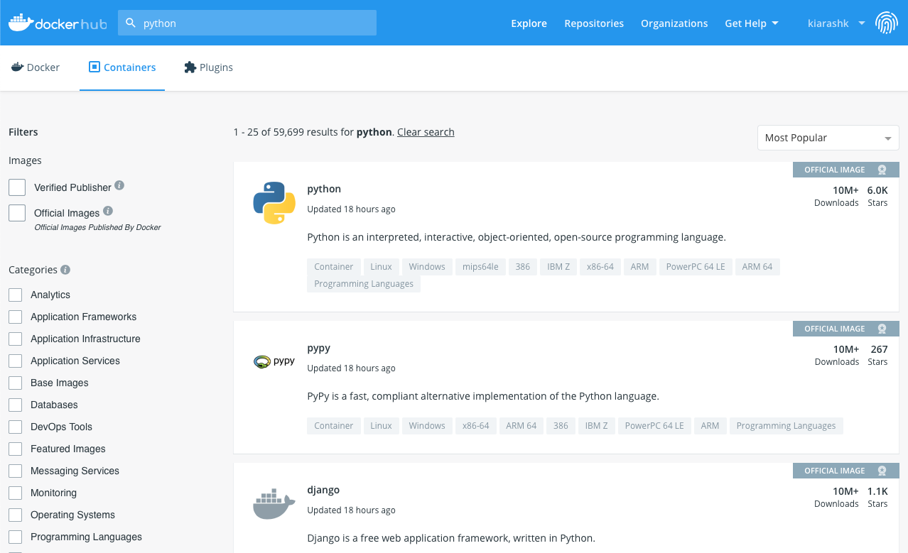
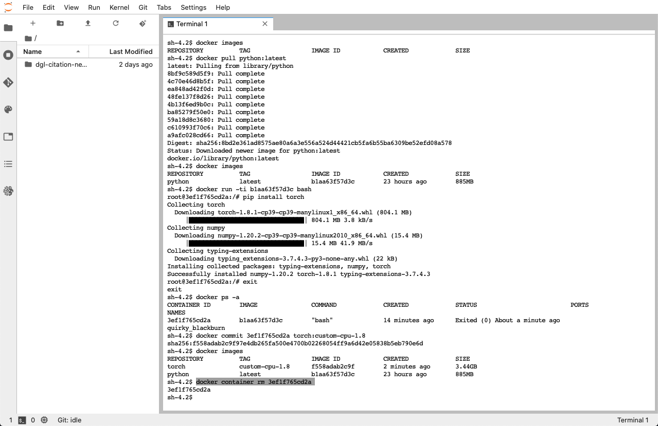
After choosing the right package and the right version, we can download the image on our SageMaker Notebook Lab by pull command:
docker pull python:latest
In docker names, what comes after the colon, defines the image version.
Now we can make a container out of it and customize it. The -ti argument means to run it in terminal interactive mode, and the bash means to run the bash application as soon as the container instantiate is up.
docker run -ti <IMAGE ID> bash
Now we are inside the container. We can update the pip and then install the last version of the PyTorch CPU version using pip. First upgrade linux package lists:
apt-get update
Now installing torch using pip:
pip install torch
By typing the command exit and hit enter, we will exit the container, and it will be stopped. Now we have updated and installed PyTorch. We are ready to commit our base image. To get the container id of our customized container:
docker ps -a
with the container id, we are able to commit our customized container to be a new docker image:
docker commit <CONTAINER ID> torch:custom-cpu-1.8
We can also clean left out containers:
docker container rm
Now that we have created our custom docker base image, we are able to deploy our model to a new image based on our customized docker image.
FROM torch:custom-1.8

RUN pip install --no-cache dgl pandas flask

COPY model.py /usr/bin/model.py
COPY train.py /usr/bin/train
COPY serve.py /usr/bin/serve

RUN chmod 755 /usr/bin/train
RUN chmod 755 /usr/bin/serve

EXPOSE 8080
The dockerfile specifies how the docker should create our new image. The following list explains each dockerfile command:
FROM: It defines what docker image should be used to build our docker image. If the image name followed by version is available locally, the docker will use the local image, and if not, the docker pulls it from the docker-hub repository.
RUN: It runs everything comes after as a bash script.
COPY: copy file from our source repository to the image.
EXPOSE: open a port to be used by our Flask web server.
SageMaker will create a new container from our image and call the train module as “train” and not “train.py” when we call the fit method of the Estimator. Therefore, we must rename train.py to train when copying it into the Dockerfile–as well as serve.py.
Auto-Deploy using Bash Script
Since it is common to face some bugs when running our custom container or we need to add/remove some features, It will be easier to put all of the bash commands for creating a docker image and pushing to ECR inside a bash file and call it instead.
#! /bin/sh
docker build -t dgl-citation-network:custom-torch-1.8 -f Dockerfile .
aws ecr get-login-password --region eu-west-1 | docker login --username AWS --password-stdin <Image URI>
docker tag dgl-citation-network:custom-torch-1.8 <Image URI>/dgl-citation-network:custom-torch-1.8
docker push <Image URI>/dgl-citation-network:custom-torch-1.8
now let’s make it executable:
chmod 755 deploy.sh
and we can run it:
./deploy.sh
Summary
We started by developing a GNN model using the DGL framework. As a way to train our model and service our predictions through AWS SageMaker, we created two Python files, one for training and saving artifacts, and one for loading the model from artifacts and serving the API. In the next step, we packaged both files into a single Docker image and uploaded it to ECR. Using SageMaker notebooks, we use the Estimator object of SageMaker SDK to automate the process of loading the image from ECR, training the model with our hyperparameters, and then serving the result.


